In which the author gets the Reversible Jump Markov Chain Monte Carlo algorithm and trans-dimension inversion off of his chest.

Posted on May 25, 2015 by wyverstein

Last time I promised to write an entry about Data Augmentation and Dispersion however I lied. The basic problem is that in order to provide an example of either process I need to first talk about Markov chain Monte Carlo (MCMC) algorithms such as Gibbs sampling or Metropolis-Hastings Sampling. And if I am going to write about MCMC then there really is no reason not to write about reversible jump Markov chain Monte Carlo (rjMCMC).

And because I talk to much and as well as desire all of these post to more or less stand on their own we shall start by reviewing statistical inversion (parameter estimation). Forward and inverse problems may be broadly defined as data prediction and parameter estimation, respectively. That is, if the function $f$ represents the process of interest (e.g., the systematic part of the KPI) and ${\bf m}$ is a vector of model parameters representing the system (predictors), then calculating predicted data ${\bf d} = f({\bf m})$ represents the forward problem, while solving the same system of equation with an observed data set ${\bf d}_0$ for an estimate of the parameters $\hat{{\bf m}}$ is the inverse problem, i.e., $\hat{{\bf m}} = f^{-1}({\bf d}_0)$ . Note, however, an analytic form for $f^{-1}({\bf d}_0)$ rarely exists and consequently the distribution of $\hat{{\bf m}}$ can only be expressed numerically.

The most common sampling paradigm is Metropolis-Hasting (MH) sampling, which produces a random walk through the parameter space. The walk is conducted such that the long-run distribution of the steps converge to the target distribution, e.g., the PPD. Figure 1 shows an example of MH sampling for a one-dimensional target distribution; the distribution of the steps converge to the target as the sampling progresses.

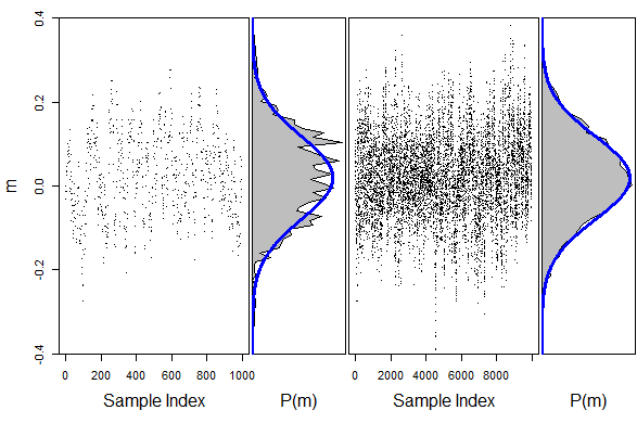
Figure 1: Samples (dots) and distribution for Metropolis-Hasting sampling after 1,000 (left) and 10,000 (right) iterations. The blue line indicates the target distribution and the shaded area is the sampled distribution.

The r code for this example is shown below; in summary the algorithm has 3 steps. These are draw the proposed model, accept or reject the proposed model, and save the model. Starting with the first step the proposed model ${\bf m'}_t$ is drawn randomly from the distribution $Q({\bf m'}_t|{\bf m}_t)$ which as the notation suggests can only depend on constants and the current model (this is not precisely true but is a simplifying lie). The second step has two parts (this is apparently distinct from there being four steps with one part each…); the first part is to calculate the acceptance probability, the other is to accept the proposed model with that probability. The acceptance probability is

where $\mathcal{L}$ is the likelihood and $\pi$ is the prior. If the proppsed model is accepted then ${\bf m}_{t+1} = {\bf m'}_t$ else ${\bf m}_{t+1} = {\bf m}_t$ . In the final step ${\bf m}_{t+1}$ is saved.

The rjMCMC is described after this code segment.

g.MCMC<-function(N= 10000)
{
# this stuff is to start the process
data = rnorm(100, mean=0, sd=1) # the simulated data mean forced to be
M = c(-Inf, 0) # starting model (log likelihood, m)
Q.mu1 = 0.05 # perterbation SD (chosen here to be bad for plotting !)
SAMPLES = M

# plot stuff
par(mar = c(0.1, 0.1, 0.1, 0.1) )
layout(mat = matrix(c(7,7,7,7,7,5,1,2,3,4,6,6,6,6,6), nrow=3, ncol=5, byrow=T),
widths = c(0.3, 1, 0.5, 1, 0.5), heights = c(0.05, 1, 0.2) )
M.frame = seq(-0.4, 0.4, length.out = 1001)
Target = dnorm(M.frame, mean= mean(data), sd=1/sqrt(length(data))) # the target distribution

# the prior
LB = -3
UB = 3

# the sampling
for (i in 1:N)
{
M.prime = M # Step 1 the proposal of a new model
M.prime[2] = M.prime[2] + rnorm(1, mean = 0, sd = Q.mu1) # the perterbation

# calculate the likelihood of the data
e          = data – M.prime[2]                  # the residuals
LL         = dnorm(e, mean=0, sd = 1, log = T ) # the log likelihood
M.prime[1] = sum(LL)                            # add LLs to get total log likelihood

# Step 2 MCMC acceptance
r = runif(1)
A = exp(M.prime[1]-M[1])
if (is.na(A)) {A= 0}
if ((A>=r)&(M.prime[2]>= LB)&(M.prime[2]<= UB))
{
M = M.prime
}
# Step 3 record sample
SAMPLES = rbind(SAMPLES, M)
rownames(SAMPLES) = NULL

if (i == 1000)
{
SAMPLES=SAMPLES[1:1000,]
# plot PPD
plot(1:1000,SAMPLES[,2], pch=”.”, yaxs=”i”, ylim=c(-0.4, 0.4), xlab=”Sample Index”, ylab=”m”)
axis(1, at = 500, tick = F, label = “Sample Index”, cex.axis=1.5, mgp=c(3, 3, 0))
axis(2, at = 0, tick = F, label = “m”, cex.axis=1.5, mgp=c(3, 3, 0))
H=hist(SAMPLES[,2], breaks=seq(min(SAMPLES[,2]),max(SAMPLES[,2]), length.out=51), plot=F)
plot( seq(0, 1.04*max(H$den), length.out=length(H$mids)),H$mids, type=”n”, xaxs=”i”, ylab=””,
xlab=””, yaxs=”i”, yaxt=”n”, xaxt=”n”, ylim=c(-0.4, 0.4))
axis(1, at = mean( seq(0, 1.04*max(H$den), length.out=length(H$mids))), tick = F, label = “P(m)”, cex.axis=1.5, mgp=c(3, 3, 0))
polygon( c(0, H$den, 0), c(-0.4, H$mids, 0.4), col=”grey”)
lines( Target, M.frame, col=”blue”, lwd=3)
}
if (i == N)
{
# plot PPD
plot(1:N,SAMPLES[,2], pch=”.”, yaxs=”i”, ylim=c(-0.4, 0.4), xlab=”Sample Index”, ylab=”m”, yaxt=”n”)
axis(1, at = N/2, tick = F, label = “Sample Index”, cex.axis=1.5, mgp=c(3, 3, 0))
H=hist(SAMPLES[,2], breaks=seq(min(SAMPLES[,2]),max(SAMPLES[,2]), length.out=51), plot=F)
plot( seq(0, 1.04*max(H$den), length.out=length(H$mids)),H$mids, type=”n”, xaxs=”i”, ylab=””,
xlab=””, yaxs=”i”, yaxt=”n”, xaxt=”n”, ylim=c(-0.4, 0.4))
axis(1, at = mean( seq(0, 1.04*max(H$den), length.out=length(H$mids))), tick = F, label = “P(m)”, cex.axis=1.5, mgp=c(3, 3, 0))
polygon( c(0, H$den, 0), c(-0.4, H$mids, 0.4), col=”grey”)
lines( Target, M.frame, col=”blue”, lwd=3)
}

}
}
g.MCMC()

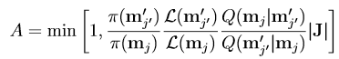
So far we have only considered cases where the number of parameters is known(i.e., the dimension of the PPD fixed), however in many setting the number of parameters is not know a priori. In such cases it may be possible to calculate the evidence for each model and select the best one, but in common applications situation that can be computationally impractical. In addition even if it is possible the point estimate for the dimension of the PPD will have uncertainty that will not be accounted for in the parameter estimate uncertainties! The rjMCMC algorithm solves both these problems. The PPD is expanded to span multiple dimensions (numbers of parameters). Like the MCMC algorithm rjMCMC takes a random walk though the parameter space but now the walk can not only perturb the parameter values but “Birth” and “Death” sets if parameters. The rjMCMC acceptance probability is
.
The time subscript (t) has been suppressed for clarity. The subscript $j$ indicates the dimension of the model vector ${\bf m}$ . The term |J| is the Jacobin of the diffeomorphism of the transform between dimension j and j’. In general if only the parameters that are birthed or deathed are altered if the dimension changes this will be 1 and be ignored. Also the proposal distribution Q can really be thought of as three parts the birth proposal, the death proposal and the perturbation proposal; i.e.,

The proposal distributions will operate in pares as the reverse move for a perturbation must be a perturbation, a birth must pare with a death, and a death with a birth. Also, in general the prior ratio will change only by the prior of the birthed / deathed parameters. Thus if the birthed parameters are proposed from the prior The acceptance probability becomes that of the standard MCMC.

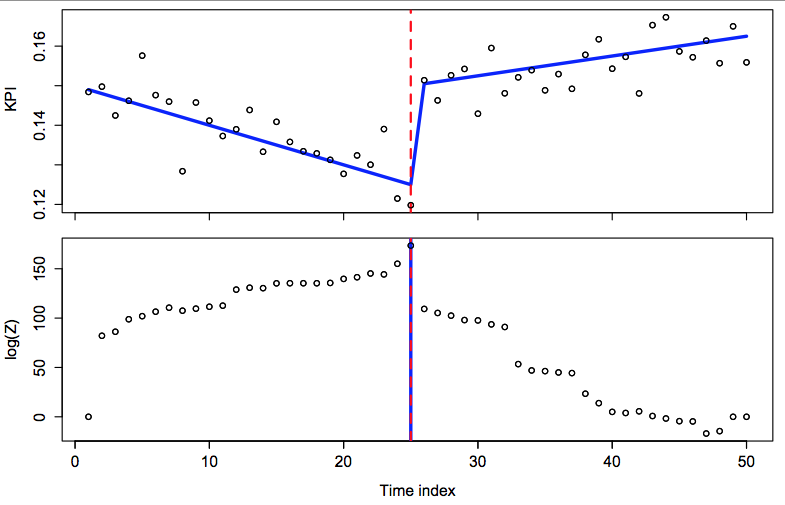
To illustrate the rjMCMC algorithm consider the following regression example. It conists of regressing 20 y’s onto 20 x’s. The order of the model is unknown, i.e., it could be a constant, linear, or quadratic. The data and true model (linear) is shown in the next figure.

The simulated noisy (circles) and true (blue line) data used inthe rjMCMC example.

The posterior uncertainty of the parameters is shown in the histograms below. Note the PPD might be under-sampled but i wanted the code to run relatively quickly and I do not want my out put to look different from your s when you run it! Out of the 25000 samples models 7595 had only a constant, 17376 had a mean and linear trend and only 28 had a quadratic term! the code for this is below.

The posterior marginal uncertainties of beta0, beta1, and beta2, the regression parameters. The dashed vertical blue lines indicate the “true” values.

To recap Bayesians commonly approximate the PPD with samples. These samples can be gathered by MCMC type algorithms. It is possible to collect the samples even if the number of model parameters are unknown. And the rjMCMC algorithm selects parameters from models proportionally to their evidence. Finally parameter uncertainties account for model selection uncertainties!

Tune in next time for Bayesian BI! Also I recently moved to Hothead games so check out our products if you get a chance (Boom Boom Soccer and Boom Boom Foot Ball are in soft launch so please play them and leave any comments you have!)

P.S. I have noticed that this blog format changes some of the symbols in the code if you have trouble running it leave a comment and I will email you directly.
The rjMCMC code:
g.predict<-function(Mod, X)
{
j = Mod[2]
beta0 = Mod[3]
beta1 = Mod[4]
beta2 = Mod[5]

P = 0*X + beta0
if (j >= 2) {P = P + X*beta1}
if (j >= 3) {P = P + (X^2)*beta2}

return(P)
}

g.perterb<-function(M=c(-Inf, 3, 0, 0, 0), Qsd=c(0, 0, 0.1, 0.01, 0.001), LB = c(0, 1, -10, -2, -1 ), UB = c(0, 1, 10, 2, 1 ) , data=data.frame(1:100, rnorm(100)))
{
# unpacking hte parameters
LL    = M[1]
j     = M[2]
#beta0 = M[3]
#beta1 = M[4]
#beta2 = M[5]
x     = data[,1]
y     = data[,2]

ORDER = sample(3:(3+j-1), j)

for (i in ORDER)
{
M.prime = M # make the proposal model
M.prime[i] = M.prime[i] + rnorm(1, mean = 0, sd= Qsd[i]) # add random noise to old model
P = g.predict(M.prime, x) # get predicted values