Rotated MCMC Sampling and Ordered Categorical Regression

Hi All

So a few times I have said something like this is not the best was to pick step distributions in MCMC but so far I have not given the my way, i.e., the best way. This post presents rotated sampling and applies it to an Order Categorical regression problem.

Rotated sampling is sampling from a transform of the parameter space. So if ${\bf m}_t$ is the current model then to get ${\bf m}_{t+1}$ first ${\bf \hat{m}}_t$ is calculated; this is done by rotating to the eigenspace of the target distribution. In the eigenspace all parameters should be uncorrelated. In addition, if the target distribution is approximately Gaussian the variances along the jth eigen vector should corresponding jth eigen values ( $\lambda_j$ ). So the proposal distribution for the jth eigen vector [ $Q(\hat{m}_j^{\prime}|\hat{m}_j)$ ] is a Gaussian with mean $\hat{m}_j$ and variance equal $0.5\lambda_j$ (The 0.5 I have for experimentally to optimize the conversion of the algorithm but I don’t think there is any magic behind it). The proposed model ( $\hat{m}_j^{\prime}$ ) is then either accepted or rejected with standard Metropolis Hastings criteria giving ${\bf \hat{m}}_{t+1}$ . The model ${\bf \hat{m}}_{t+1}$ is then rotated back to the original parameter space yielding ${\bf m}_{t+1}$ .

This may seem unsatisfying as knowledge of the eigen space of the target distribution could not be known in any realistic problem. However this loop is avoided by using burn-in samples to estimate the target distribution variance co-variance structure; i.e., the true parameter co-variance matrix ( $C_{\bf m}$ ) is estimated by the co-variance matrix of the samples $\hat{C}_{\bf m}$ . The rotation matrix $U$ and the eigen values ${\bf \lambda}$ are then found by using the singular value decomposition of $\hat{C}_{\bf m}$ .

A few notes for those of you that will actually run try to implement this. As shown in the attached code the rotation is generally done once for multiple proposals (one for each eigen vector). Also the co-variance matrix $\hat{C}_{\bf m}$ is only updated periodically. Finally fixed length sampling (see appendix C.2 in my thesis) is used to reduce the computational load.

So now on to the actual problem (these are important because without problems it is hard to justify the importance of solutions). Consider to conducting a regression with the observation being ordinal categorical variables (e.g., something like NDP, Liberal, Conservative; Group 1 > Group 2 > Group 3 but the average of a Group 1 and a Group 3 is not a Group 2). In this case it is attractive to use a latent variable model described on the wiki page. The idea is that as the systematic component/ linear predictor of the model increases the probability of being in a higher group increases and as the systematic component/ linear predictor decreases the probability of being in a lower group increases. This is vary similar to probit regression, however it requires the additional estimation of threshold values ( $\alpha_{12}$ , $\alpha_{23}$ … $\alpha_{(n-1)n}$ ). In out example with three groups The probability of a data point $d_i | \alpha_{12}, \alpha_{23}, \sigma, \eta_i$ where $\eta_i$ is the linear predictor (i.e., $\eta_i = {\bf x}_i {\bf \beta}$ ) is $\Phi([\alpha_{12} -\eta_i]/ \sigma)$ if $d_i =$ Group 1, $\Phi([\alpha_{23} -\eta_i]/ \sigma) - \Phi([\alpha_{12} -\eta_i]/ \sigma)$ if $d_i =$ Group 2, and $1 - \Phi([\alpha_{23} -\eta_i]/ \sigma)$ if $d_i =$ Group 3.

The data in this toy problem looks like Fig. 1. As $x$ grows observations are more likely to be a 2 instead of a 1 and then a 3 instead of a 2. The true parameter values for $\beta, \sigma, \alpha_{12}, and \alpha_{23}$ and 1, 1, 5, and 5 respectively. Figure 2 shows the posterior samples. Figure 3 shows a scatter plot of the posterior samples in the eigen space of the distribution. The key point looking at figs. 2 and 3 is that there is a lot of correlation in fig. 2 and none in fig. 3. The correlation makes MCMC sampling difficult but that problem is completely avoided by working in the rotated space.

Figure 1: The observed groups as a function of the predictor x.

Figure 2: A scatter plot of the posterior samples. Note the high level of correlation between the parameters.

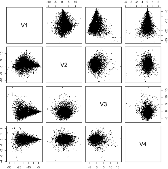
Screen Shot 2016-10-16 at 8.33.17 PM.png

Figure 3: The posterior distribution samples in eigen space. Note that lack of correlation between the eigen vectors.

That’s it for this time. Sorry for the lack of humorous links I just wanted to get this one done. To make up for it though Figure 4 is photo of Mr Fitzwilliam Darcy with a bearded dragon on him. Code is appended.

Figure 4: Mr Fitzwilliam Darcy (the cat) and Spika (The Bearded Dragon).

Code:

g.data.maker<-function(N)
{


x    = seq(-10, 10, length.out =N)
sigma = 3

n    = rnorm(N, mean = 0, sd =sigma)
beta = 1

y.star.t = beta*x
y.star = beta*x+n

alpha12 =  -5
alpha23 =  5

y = cut(y.star , breaks = c(-Inf,alpha12,alpha23, Inf  ), labels = c(1, 2, 3))

y2 = cut(y.star , breaks = c(-Inf,alpha12,alpha23, Inf  ), labels = c("B", "N", "G"))

plot(x,y, type= "n")

abline(h= alpha12, col="grey")
abline(h= alpha23, col="grey")
text(x,y, label=y2)



return(data.frame(x,n,y.star.t, y.star, y))

}


data.polr = g.data.maker(N=1000)



g.likelihood<-function(data = data.polr, m=c(1,3, -5,5)  ) { n    = nrow(data) x    = data[,1] y    = data[,5] beta    = m[1]   sigma   = m[2]   alpha12 = m[3]    alpha23 = m[4] if (alpha12 >= alpha23) {return(-Inf)}

if (abs(alpha12) >= 20) {return(-Inf)}
if (abs(alpha23) >= 20) {return(-Inf)}

#prior
P.beta     = dnorm(beta, mean = 0, sd = 5, log =T) 
P.sigma    = - sigma 
P.alpha12  = dnorm(alpha12, mean = 0, sd = 10, log =T) 
P.alpha23  = dnorm(alpha23, mean = 0, sd = 10, log =T) 


y.star.hat = x*beta

L1  = pnorm(alpha12, mean =y.star.hat, sd = sigma )
L2  = pnorm(alpha23, mean =y.star.hat, sd = sigma )


#LMAT = matrix(c(L1, L2-L1, 1-L2), ncol=3, nrow= n)
LLMAT = matrix(c(log(L1), log(L2-L1), log(1-L2)), ncol=3, nrow= n)

#print(data.frame(x,y,LMAT))

#print(LLMAT[cbind(1:n, y)])

LL = LLMAT[cbind(1:n, y)]
LL = sum(LL)

if(is.na(LL)) {LL=-Inf}

LL = LL + P.beta   + P.sigma  + P.alpha12+ P.alpha23

return(LL)


}
g.likelihood( m=c(1,3, -5,5))




g.rot<-function(v, r)
    {
    out = v%*%r

    return(out)

    }



g.REM.mcmc<-function(n, n1 ) { rot = matrix(0, nrow =4, ncol=4) diag(rot) =1 rot.inv  = rot  N.temps = 13 EX = seq(0, 3, length.out = N.temps ) t.star = 2^EX data = g.data.maker(N=100) M = matrix( nrow = N.temps, ncol= 6) for ( i in 1:N.temps)  {  ll.old = -Inf  while(ll.old == -Inf)      {      m.old = c(runif(1, min = 0.5, max = 1.5), runif(1, min = 0, max = 5), runif(1, min = -10, max = 0), runif(1, min = 0, max = 10))      ll.old = g.likelihood(m = m.old)      print(i)      print(ll.old)      }  M[i,1] = ll.old  M[i,2:5] = m.old  M[i,6] = t.star[i]  }  print(M) M.list = c(ll.old, m.old,0) alpha = 1 ll.best = ll.old m.best  = m.old P.UD = 0.01 ac.list = rep(0, 4) ac.list.temp = rep(0,4) try.list.temp = rep(0,4) j.sd = c(0.000001, 0.000001, 0.000001, 0.000001) for ( i in 1:n1)     {     # loop for each temp     #print("jump")     #print(i)      try.list.temp[1:4] = try.list.temp[1:4] +1     for(k in 1:N.temps)         {         # the the current chain         m.old     = M[k, 2:5]         t.star    = M[k, 6]         LL.old    = M[k, 1]         m.old.rot = g.rot(v=m.old, r=rot)         # MCMC step         for (j in 1:4)             {             #print(c(i,k,j))             m.new.rot     = m.old.rot             m.new.rot[j]  = m.new.rot[j] + j.sd[j]*rcauchy(1)             m.new         = g.rot(m.new.rot, r = rot.inv)               LL.new        = g.likelihood(data, m=m.new)             if (LL.new >= ll.best)
                {
                ll.best = LL.new
                m.best = m.new

                }
   
            #print(LL.new)
            #print(LL.old)
            #print(t.star)
            A = exp( (LL.new - LL.old)/t.star )
            if (is.nan(A)) {A = 0}



            #print(A)
            r = runif(1)
            if (r <=A )
                {
                m.old     = m.new
                LL.old    = LL.new
                m.old.rot = m.new.rot


                if(t.star == 1) {ac.list[j]      = ac.list[j] +1     }
                if(t.star == 1) {ac.list.temp[j] = ac.list.temp[j] +1}
                }

            #if(t.star == 1)
            #    {   
            #    print(i)
            #    print(j)
            #    print(ac.list)
            #    print(ac.list.temp)
#
            #    }
#


   
            }   

        M[k, 2:5] = m.old
        M[k, 1]   = LL.old
        }

    #print("swap")
    #print(i)
    # swap information
    r = runif(1)
     if ( (r<= 0.10) ) # clearly this (the DREM on switch) should also be in the liklihood step but i am lazy and this fast anyway
         {
         for (j in 1:100)
             {
             k = sample(x = 1:N.temps, size= 2, replace =T)
             A = exp((M[k[1],1] - M[k[2],1])*( (1/ M[k[1],6] ) - (1/M[k[2],6] ) ))
             if (is.nan(A)) {A = 0}
             r = runif(1)
             if ( r <= A)
                 {
                 T1 = M[k[1],6]
                 T2 = M[k[2],6]

                 M[k[1],6] = T2
                 M[k[2],6] = T1
                 }
             }
         }
     #print("Record")
    #print(i)

     # first samples
    if ( i <= 999)          {         M.list = rbind(M.list, c(M[M[,6]==1,1:5 ],i))         rownames(M.list) =NULL         alpha = 1         }     # fixed length thinning     if ( i > 999)
        {
        alpha = alpha*1000/(alpha+1000)
        r = runif(1)
        if ( r <= alpha)             {             row = sample(1:1000,1)             M.list[row,] = c(M[M[,6]==1,1:5 ],i)             }     }     # update j.sd      #print("Update SD")      #print(i)     r = runif(1)     #print(r)     if (( i >= 100)&(r <= P.UD))         {         print("------------------------------------------------------")         print(i)         Cm = cov(M.list[,2:5])         Q = svd(Cm)         print(Q)         j.sd = 0.5*sqrt(Q$d)         rot = Q$u         rot.inv = t(rot)         #print(Rec)         if(1==2)         {         for (i in 1:4)             {             P  = ac.list.temp[i]/try.list.temp[i]             mult  = 1+ abs(0.5-P)             if (P >= 0.5) {j.sd[i]=j.sd[i]*mult}
            if (P < 0.5) {j.sd[i]=j.sd[i]/mult}             }         }         print(j.sd)         print("Trys, accs, ratio ")            print(try.list.temp )            print( ac.list.temp )                print( ac.list.temp/try.list.temp )            print(ac.list)            print(ll.best)         print(m.best)         ac.list.temp  = rep(0,4)         try.list.temp = rep(0,4)         }     } plot(as.data.frame(M.list[,2:5]), pch=".") M.list = c(ll.best, m.best,0) ac.list       = rep(0, 4) ac.list.temp  = rep(0,4) try.list.temp = rep(0,4) t.star = 2^EX for ( i in 1:N.temps)  {  M[i,1]   = ll.best  M[i,2:5] = m.best  M[i,6]   = t.star[i]  }  print(M) for ( i in 1:n)     {     # loop for each temp     #print("jump")     #print(i)      try.list.temp[1:4] = try.list.temp[1:4] +1     for(k in 1:N.temps)         {         # the the current chain         m.old     = M[k, 2:5]         t.star    = M[k, 6]         LL.old    = M[k, 1]         m.old.rot = g.rot(v=m.old, r=rot)         # MCMC step         for (j in 1:4)             {             #print(c(i,k,j))             m.new.rot     = m.old.rot             m.new.rot[j]  = m.new.rot[j] + j.sd[j]*rcauchy(1)             m.new         = g.rot(m.new.rot, r = rot.inv)               LL.new        = g.likelihood(data, m=m.new)             if (LL.new >= ll.best)
                {
                ll.best = LL.new
                m.best = m.new

                }
   
            #print(LL.new)
            #print(LL.old)
            #print(t.star)
            A = exp( (LL.new - LL.old)/t.star )
            if (is.nan(A)) {A = 0}



            #print(A)
            r = runif(1)
            if (r <=A )
                {
                m.old     = m.new
                LL.old    = LL.new
                m.old.rot = m.new.rot


                if(t.star == 1) {ac.list[j]      = ac.list[j] +1     }
                if(t.star == 1) {ac.list.temp[j] = ac.list.temp[j] +1}
                }

            #if(t.star == 1)
            #    {   
            #    print(i)
            #    print(j)
            #    print(ac.list)
            #    print(ac.list.temp)
#
            #    }
#


   
            }   

        M[k, 2:5] = m.old
        M[k, 1]   = LL.old
        }

    #print("swap")
    #print(i)
    # swap information
    r = runif(1)
     if ( (r<= 0.10) ) # clearly this (the DREM on switch) should also be in the liklihood step but i am lazy and this fast anyway
         {
         for (j in 1:100)
             {
             k = sample(x = 1:N.temps, size= 2, replace =T)
             A = exp((M[k[1],1] - M[k[2],1])*( (1/ M[k[1],6] ) - (1/M[k[2],6] ) ))
             if (is.nan(A)) {A = 0}
             r = runif(1)
             if ( r <= A)
                 {
                 T1 = M[k[1],6]
                 T2 = M[k[2],6]

                 M[k[1],6] = T2
                 M[k[2],6] = T1
                 }
             }
         }
     #print("Record")
    #print(i)

     # first samples
    if ( i <= 9999)          {         M.list = rbind(M.list, c(M[M[,6]==1,1:5 ],i))         rownames(M.list) =NULL         alpha  = 1          }     # fixed length thinning     if ( i > 9999)
        {
        alpha = alpha*10000/(alpha+10000)
        r = runif(1)
        if ( r <= alpha)             {             row = sample(1:10000,1)             M.list[row,] = c(M[M[,6]==1,1:5 ],i)             }     }     # update j.sd      #print("Update SD")      #print(i)     r = runif(1)     #print(r)     if (( i >= 100)&(r <= P.UD))
        {



        print("------------------------------------------------------")
        print(i)
        print("SD")
        print(j.sd)
        print("Trys, accs, ratio ")   
        print( try.list.temp )   
        print( ac.list.temp )       
        print( ac.list.temp/try.list.temp )  
        print(" total accs") 
        print(ac.list)   
        print("Best")
        print(ll.best)
        print(m.best)


        if(sum(ac.list.temp) == 0)
            {
            print(M)

            }


        ac.list.temp  = rep(0,4)
        try.list.temp = rep(0,4)

        }








    }

quartz()

samps1 = as.data.frame(M.list[,2:5])
colnames(samps1) = c("Beta", "Sigma", "Alpha12", "Alpha23")
plot(samps1, pch=".")

quartz()

plot(as.data.frame(M.list[,2:5]%*%rot), pch=".")

#par(mfrow= c(5,1), mar=c(1,4,1,1))
#plot(M.list[,1])
#plot(M.list[,2])
#plot(M.list[,3])
#plot(M.list[,4])
#plot(M.list[,5])


return(M.list)


}

samp = g.REM.mcmc(n=50000, n1 =100000)

1 thought on “Rotated MCMC Sampling and Ordered Categorical Regression”

Pingback: An ordered categorical regression approach to rating chess players. | Bayesian Business Intelligence

Bayesian Business Intelligence

Bayesian Statistical Techniques for Business Intelligence and Data Science

Rotated MCMC Sampling and Ordered Categorical Regression

1 thought on “Rotated MCMC Sampling and Ordered Categorical Regression”

Leave a Reply Cancel reply

Share this:

Like this:

Related

1 thought on “Rotated MCMC Sampling and Ordered Categorical Regression”

Leave a Reply Cancel reply